Uncategorized | Shanxiang Lyu

Archive for Uncategorized

Approximate message passing (AMP) for Massive MIMO detection, MATLAB codes provided

December 4, 2015 Uncategorized No comments

In this exposition, we want to highlight that the approximate message
passing (AMP) has superior complexity when serving the Massive MIMO
uplink detection, although AMP was initially proposed for solving a
LASSO problem [DMM09]. Regarding expository detail about why AMP
works, please see [BM11].

Regarding the problem of Massive MIMO uplink detection [HBD13], the
architecture serves tens of users by employing hundreds of antennas,

$\bm{y}=\bm{H}\bm{x}+\bm{w}$

where the channel $\bm{H}\in\mathbb{C}^{m\times n}$ has its elements
sampled from $\mathrm{\mathcal{N}}_{\mathbb{C}}(0,1/m)$ , $m\gg n$ ,
$\bm{y}\in\mathbb{C}^{m}$ is the received signal, AWGN noise components
$w_{i}$ are i.i.d with $\mathrm{\mathcal{N}}_{\mathbb{C}}(0,\sigma^{2})$ ;
regarding the transmitted $\bm{x}$ , we only assume that it’s zero
mean and finite variance $\sigma_{s}^{2}$ .

Before incorporating the AMP algorithm, we should be well aware of
two facts: 1. directly using maximum a priori (MAP)
$\arg\max\thinspace p(\bm{x}|\bm{y})$ or MMSE estimation
$\mathbb{E}_{p(\bm{x}|\bm{y})}(X)$ to work with the exact prior
degrade the necessity of employing AMP, because achieving a full
diversity requires an extremely large set of constellation points, in
which AMP works slowly while doing the moment matching process, not
to mention problems about its inability to converge to the lowest
fixed point. 2. In the CDMA multiuser detection theory [Verdu98,
etc.], their “MMSE” detector does not mean the one working with
exact prior , but rather the one assuming a Gaussian prior.

So we use a proxy prior for detecting $\bm{x}$ , i.e., assuming that
$x_{i}\sim\mathrm{\mathcal{N}}_{\mathbb{C}}(0,\sigma_{s}^{2})$ , and it will result in a MAP function that is statistically extremely close to the true MAP in Massive MIMO. In this occurrence, we have the signal power
$\sigma_{s}^{2}=2$ in QPSK, $\sigma_{s}^{2}=10$ in 16QAM, etc. So
the target function becomes:

$\min\left\Vert \bm{y}-\bm{H}\bm{x}\right\Vert ^{2},\thinspace s.t.\thinspace x_{i}\sim\mathrm{\mathcal{N}}_{\mathbb{C}}(0,\sigma_{s}^{2})$

The AMP algorithm to solve the above problem only requires three
lines (see [BM11], or our next paper which delivers a universal
version of this algorithm):

(1) $\begin{equation*} \bm{r}^{t}=\bm{y}-\bm{H}\bm{x}^{t-1}+\frac{n}{m}\frac{\sigma_{s}^{2}}{\sigma_{s}^{2}+\alpha^{t-1}}\bm{r}^{t-1} \end{equation*}$

(2) $\begin{equation*} \alpha^{t}=\sigma^{2}+\frac{n}{m}\frac{\alpha^{t-1}\sigma_{s}^{2}}{\sigma_{s}^{2}+\alpha^{t-1}} \end{equation*}$

(3) $\begin{equation*} \bm{x}^{t}=\frac{\sigma_{s}^{2}}{\sigma_{s}^{2}+\alpha^{t}}(\bm{H}^{*}\bm{r}^{t}+\bm{x}^{t-1}) \end{equation*}$

where the initialization is to let $\bm{r}^{0}=\bm{0}$ , $\bm{x}^{0}=\bm{0}$ ,
$\alpha^{0}=\sigma_{s}^{2}$ . In terms of complexity, it only costs
$2mn\times\mathrm{(\#Iteration)}$ . Also, according to the second
equation of the algorithm, it is converging extremely fast. On the
contrary, MMSE has complexity $O(mn^{2})$ . It is noteworthy that
known approximation methods to MMSE, such as Richardson’s method or
Newman series approximation, both fall behind the complexity-performance
trade-off of AMP according to our simulations.

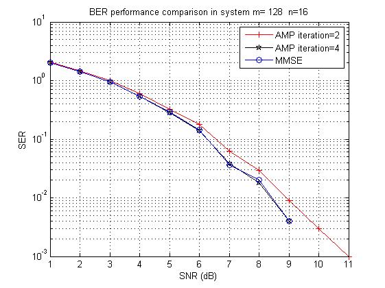
Now we share simulation results as well as MATLAB source codes.

%   AMP detector in Massive MIMO
%   written by Shanxiang Lyu (s.lyu14@imperial.ac.uk)
%   Last updated on 04/12/2015
function main()
clc;clear; close all; 
m=128;% # of received antennas
n=16;% # of users
SNRrange=[1:20];
count=0;
for s=SNRrange
SNRdb=s;
    for monte=1:1000
    x=(2*randi([0,1],n,1)-ones(n,1))+sqrt(-1)*(2*randi([0,1],n,1)-ones(n,1));
    sigmas2=2;%signal variance in QPSK
    H=1/sqrt(2*m)*randn(m,n)+sqrt(-1)/sqrt(2*m)*randn(m,n);
    sigma2=2*n/m*10^(-SNRdb/10); %noise variance in control by SNR in DB
    w=sqrt(2*sigma2)*randn(m,1)+sqrt(-1)*sqrt(2*sigma2)*randn(m,1);
    y=H*x+w; %channel model

    %iterAMP is # of iterations in AMP
    iterAMP1=2;
    xhat1=AMP(y,H,sigma2,sigmas2,iterAMP1,m,n);
     iterAMP2=4;
    xhat2=AMP(y,H,sigma2,sigmas2,iterAMP2,m,n);
    
     x_mmse=(sigma2/sigmas2*eye(n)+H'*H)^(-1)*H'*y;
     x_mmse=sign(real(x_mmse))+sqrt(-1)*sign(imag(x_mmse));
    errorAMP1(monte)=sum(x~=xhat1);
    errorAMP2(monte)=sum(x~=xhat2);
    errorMMSE(monte)=sum(x~=x_mmse);
    end
    count=count+1;
serAMP1(count)=mean(errorAMP1);
serAMP2(count)=mean(errorAMP2);
serMMSE(count)=mean(errorMMSE);
end
figure(1)% plot the SER
semilogy(SNRrange,serAMP1,'-+r', SNRrange,serAMP2,'-pk',SNRrange, serMMSE,'-ob'); 
grid on;
legend(['AMP iteration=' int2str(iterAMP1)], ['AMP iteration=' int2str(iterAMP2)], 'MMSE');
xlabel('SNR (dB)'); ylabel('SER');
title(['BER performance comparison in system m= ' int2str(m)  '  n=' int2str(n)]);
end
function xhat=AMP(y,H,sigma2,sigmas2,iterAMP,m,n)
%   AMP detector in Massive MIMO
%   written by Shanxiang Lyu (s.lyu14@imperial.ac.uk)
%   Last updated on 04/12/2015
    r=zeros(m,1);
    xhat=zeros(n,1);
    alpha=sigmas2;%initial estimation variance
        for t=1:iterAMP
        r=y-H*xhat+(n/m)*sigmas2/(sigmas2+alpha)*r;
        alpha=sigma2+(n/m)*sigmas2*alpha/(sigmas2+alpha);
        xhat=(sigmas2/(sigmas2+alpha))*(H'*r+xhat);
        end
    xhat=sign(real(xhat))+sqrt(-1)*sign(imag(xhat));
end

On cryptography and web-security

October 2, 2015 Uncategorized No comments

To spare the hours doing my PHD, I am recently watching the cryptography online courses provided by Prof. Dan Bobeh. For those who may be interested in what “cryptography” and “web-security” are doing, I have drawn two figures to highlight my understanding.

Showing the decoding radius of SIC is larger than that of ZF

April 27, 2015 Uncategorized No comments

Zero forcing (ZF) and successive interference cancellation (SIC) are among the most popular sub-optimal approaches to perform a MIMO detection. Ref. [1] serves as a great analytic perspective to look at the decoding radius of ZF, SIC and their lattice reduction counter parts. However, the statement about the size comparison of SIC and ZF decoding radius is still away from ‘nice and clear’, i.e.,

(pp. 2799, para 2 on the left column)”Since $\hat{b}_i$ only needs to be orthogonal to ${b}_1, \ldots,b_{i-1}$ , we must have $\theta_i\leq\phi_i$ and hence $d_{i,ZF}\leq d_{i,SIC}$ “.

In this post, we try to establish a proof about “ $d_{i,ZF}\leq d_{i,SIC}$ “.

First of all, necessary notations are given, as those in Ref. [1]. Let $d_{i,ZF}$ be the Euclidean distance from point $0$ to the $i$ -th facet of the decision regions of ZF and SIC, respectively. Then the distance spectrum of them are given by:

$d_{i,ZF}=\frac{1}{2}||\mathbf{b}_i||\sin \theta_i\\ d_{i,SIC}=\frac{1}{2}||\mathbf{b}_i||\sin \phi_i$

where $\theta_i$ denotes the angle between $\mathbf{b}_i$ and the space span by all the rest columns of matrix $\mathbf{B}$ , and $\phi_i$ is the angle between $\mathbf{b}_i$ and the space span by the columns before $i$ . We dubs the two notations as

$\theta_i=angle(\mathbf{b}_i,span(\mathbf{B_{[-i]}))$

$\phi_i=angle(\mathbf{b}_i,span(\mathbf{B_{[1\sim i-1]}))$

In order to show that $\sin \theta_i \leq \sin \phi_i$ , it is indeed showing

$\frac{||Proj(\mathbf{b}_i,span^\perp (\mathbf{B}_{[-i]}))||}{||\mathbf{b}_i||}\leq\frac{||Proj(\mathbf{b}_i,span^\perp (\mathbf{B}_{[1\sim i-1]}))||}{||\mathbf{b}_i||}$

where the “Proj” operator means taking the projection of vectors onto their orthogonal complement. Let the normalized Gram-Schmidt basis of $\mathbf{B}$ note as $\hat{\mathbf{B}}=[\hat{\mathbf{b}}_1,...,\hat{\mathbf{b}}_n]$ , then we have

${||Proj(\mathbf{b}_i,span^\perp (\mathbf{B}_{[-i]}))||}= ||\hat{\mathbf{B}}_{i}\hat{\mathbf{B}}_{i}^{\mathrm{T}}\mathbf{b}_i||$

${||Proj(\mathbf{b}_i,span^\perp (\mathbf{B}_{[1\sim i-1]}))||}= ||\hat{\mathbf{B}}_{[i\sim n]}\hat{\mathbf{B}}_{[i\sim n]}^{\mathrm{T}}\mathbf{b}_i||$

where $||\hat{\mathbf{B}}_{i}\hat{\mathbf{B}}_{i}^{\mathrm{T}}\mathbf{b}_i||=||\hat{\mathbf{b}}_{i}\hat{\mathbf{b}}_{i}^{\mathrm{T}}\mathbf{b}_i||$ and $||\hat{\mathbf{B}}_{[i\sim n]}\hat{\mathbf{B}}_{[i\sim n]}^{\mathrm{T}}\mathbf{b}_i||= ||\hat{\mathbf{b}}_{i}\hat{\mathbf{b}}_{i}^{\mathrm{T}}\mathbf{b}_i+$ $\hat{\mathbf{b}}_{i+1}\hat{\mathbf{b}}_{i+1}^{\mathrm{T}}\mathbf{b}_i+\ldots+\hat{\mathbf{b}}_{n}\hat{\mathbf{b}}_{n}^{\mathrm{T}}\mathbf{b}_i||$ , among which the vectors are pair-wise orthogonal. Thus $||\hat{\mathbf{B}}_{i}\hat{\mathbf{B}}_{i}^{\mathrm{T}}\mathbf{b}_i||\leq||\hat{\mathbf{B}}_{[i\sim n]}\hat{\mathbf{B}}_{[i\sim n]}^{\mathrm{T}}\mathbf{b}_i||$ , and we arrive in the conclusion that

$\sin \theta_i\leq \sin \phi_i$

So the decoding radius of SIC is larger.

References:

[1] C. Ling, “On the proximity factors of lattice reduction aided decoding”, IEEE Transactions on signal processing, Vol.59, No.6, pp. 2795–2808, 2011.

[2] Y.H. Gan, C. Ling and W.H. Mow, “Complex lattice reduction algorithm for low-complexity full-diversity MIMO detection”, IEEE Transactions on signal processing, Vol.57, No.7, pp. 2701–2710, 2009.

How to separate a graph? A first look at spectral method.

April 20, 2015 Uncategorized No comments

Planted partition can be intuitively regarded as, literally, separating a graph according to your plan. The problems such as bisection, k-coloring and maximum clique are known to be hard, and actually, most problems are hard unless proven easy.

In this post, we firstly try to classify the spectral graph model, and then given out the matlab code for partitioning a bipartite graph.

A general model for structural graph is:

$\mathcal{G}(\psi,P)$ : let $\psi: \{ 1,\ldots,n\}\rightarrow \{ 1,\ldots,k\}$ which meaning the mapping from vertices to classes, and $P$ be its generating matrix of size $k\times k$ , where $P_{i,j}\in\{0,1\}$ . So the connecting probability of any edge $(u,v)$ is $P_{\psi(u),\psi(v)}$ .

So the weighted adjacency matrix of $\mathcal{G}(\psi,P)$ looks like

$\left( \begin{array}{cccc} P_{1,1}& P_{1,1}& P_{1,2}& P_{1,2}\\ P_{1,1}& P_{1,1}& P_{1,2}& P_{1,2}\\ P_{1,2}& P_{1,2}& P_{2,2}& P_{2,2}\\ P_{1,2}& P_{1,2}& P_{2,2}& P_{2,2} \end{array} \right)$ ,

where the symmetric property of this matrix descents from that it is an in-directed graph.

We further specialize the bisection model hereby

Planted Bisection $(\psi,p_1,p_2,q)$ : the connecting probability of connecting to its own section is $p_1$ and $p_2$ respectively, while that of crossing is $q$ .

Suppose we are now given a graph of this form, and want to simulate the process of partitioning all these nodes into two sections, with least possible crossing edges. Before delving into those technical details, we briefly describe a spectral partitioning principle for our simulation in this post:

The eigenvector of the second largest eigenvalue of the adjacency matrix $\mathbf{A}$ is a slightly perturbed version of its generator matrix $\mathbf{M}$ , which is of the form

$\mathbf{M}=$ $\left( \begin{array}{cccc} p_1 & p_1 & q & q \\ p_1 & p_1 & q & q \\ q & q & p_2 & p_2 \\ q & q & p_2 & p_2 \\ \end{array} \right)$ .

Now we run a MATLAB simulation to simulate how that spectral partitioning method works.

Generate a graph with $n$ vertexes, and $n_1$ vertexes are connecting each other with probability $p_1$ , while the other $n-n_1$ vertexes are self connecting with probability $p_2$ . And that of their crossing is $q$ .

clc;clear all;
n=800;
x=randperm(n);%put the sets among random positions
n_1=round(n/4);
ind_set1=x(1:n_1);
ind_set2=x(n_1+1:end);
p_1=0.8;
p_2=0.8;
q=0.001;
A(ind_set1,ind_set1)=rand(n_1,n_1)<p_1;
A(ind_set2,ind_set2)=rand(n-n_1,n-n_1)<p_2;
A(ind_set1,ind_set2)=rand(n_1,n-n_1)<q;
A(ind_set2,ind_set1)=rand(n-n_1,n_1)<q;
A=triu(A,1);%to make the adjacency matrix symmetric
A=A+A';
figure(1)
spy(A);

When this graph is generated, we can hardly tell any relation among its connection according to figure 1.

Again, we should bear in mind that the second eigenvector $\mathbf{v}_2$ of $\mathbf{A}$ is a perturbed version of $\mathbf{w}_2$ of the generator matrix $\mathbf{M}$ . (means the values of $\mathbf{v}_2$ are just a little deviated from $\mathbf{w}_2$ ) And why is $\mathbf{w}_2$ this important? because it is of the form $[k_1p_1,k_1p_1,k_2p_2,k_2p_2,k_2p_2,k_1p_1]$ , which reflects the relation of all these vertexes. So our second step of the code is

Get the second eigenvector of $\mathbf{A}$ , and re-sort the positions of these $n$ vertexes.

[V D] = eigs(A, 2);
[useless ind_recover] = sort(V(:,2));
A_hat=A(ind_recover,ind_recover);
figure(2)
spy(A_hat);

Then we can see from figure 2 below that the relation it reflects is really a bisection.

References:

1. Daniel A. Spielman, “Spectral partitioning in the planted partition model”, Lecture notes(Lecture 21), 2009.

2. Frank McSherry, “Spectral partitioning of random graphs”, STOC, 2001.

3. David Gleich, “Spectral Graph Partitioning and the Laplacian with Matlab”, 2006. (Online resources)

Archive for Uncategorized

Approximate message passing (AMP) for Massive MIMO detection, MATLAB codes provided

On cryptography and web-security

Showing the decoding radius of SIC is larger than that of ZF

How to separate a graph? A first look at spectral method.

Shanxiang Lyu

Ph.D. of post-quantum cryptography

Search in this site

Recent Posts

Pages