BRIEF

Prototype is a well-established engineering concept to have thorough understanding, design evaluation and outcome inspection. Utilizing everything in recursive and optimized fashion, final Algorithm/Structure/Model emerges as the most practical candidate for actual/true implementation.

Software Prototyping (Simulation) is the most recent, highly effective and flexible with minimal cost & time benefits. Out of a known set of algorithms or new variants of existing algorithms that might have seemed potential enough must be tested/simulated to highlight their own advantages and limitations under various degrees of synthetic environment. They all have to be judged in all respects with actually implemented and proven algorithms to open up new directions!

Even the selection of a simulation language or a package is also as crucial as the algorithm. Features like availability, reliability, easy to use, user-friendly help, fast execution and the most important is its ability to provide directly or programmatically all complex and application specific constructs needed for the simulation of interest.

In case of SAR Imaging, a small portion of the illuminated ground patch at a given time with a resolution of interest is considered a Point Target. The key element for ground imaging is a point target because a given ground patch of illumination can be viewed as a two-dimensional grid of several point targets. An algorithm which works well for a point target has to work satisfactorily for a given ground patch and hence for an entire swath.

There are three major algorithms for Azimuth Processing (Correlation) to achieve desired Azimuth Resolution.

1 Time-Domain Azimuth Signal Processing (TASP)

2 Frequency-Domain Azimuth Signal Processing (FASP)

2.1 Time Weighted FASP (TW-FASP)

2.2 Frequency Weighted FASP (FW-FASP)

3 Spectral Analysis (SPECAN)

In this Section, the underlying core essence are tried to be presented…

1 MATLAB as a powerful simulation tool.

2 Importance of a point target in calibration of SAR processing algorithms.

3 End-to-end design understanding and verification of actually implemented Time-Domain algorithm with the help of MATLAB simulation.

4 An approach to a Frequency-Domain algorithm with two innovative ideas of Weighting in Time and Weighting in Frequency.

5 Results of Time-Domain & Frequency-Domain simulations and a comparative study of various outcomes and interpretations.

For both Time-Domain & Frequency-Domain Azimuth Signal Processing simulations in MATLAB, certain assumptions are followed to avoid unnecessary complexities.

· Point target geometry in context to Air-borne SAR in Slant Range.

· Ideal, stable radar platform with no spatial motion, straight- linear flight path of air-craft with constant velocity.

· Uniform illumination & scattering for the ground patch and symmetrical horizontal & vertical Beam-width of a Monostatic Antenna.

· No RCMC (Range Cell Migration Correction).

· No Radiometric and Geometric Correction.

Selected parameters for a given system and various formats of Azimuth Resolution & ISLR for both the simulations with ideal & noisy conditions are shown here as look ahead clues.

Requirements:

Azimuth Resolution: At least 6m or better.

ISLR (dB): Maximum (in absolute form) as possible.

System Parameters:

Antenna Length: 1.3 m, Antenna Width: 8 to 9 cm

Antenna Look Angle: » 60°

Air-craft Velocity: 120 m/s, Air-craft Altitude: 6000 m

Center Frequency/ Wavelength of Transmitted Chirp: 5.3GHz/ 5.6cm

Shortest Slant Range: 8000 m, Longest Slant Range: 32,000 m

Swath-width: 25000 m

Processing Bandwidth for given Resolution: 20Hz+ dbw tolerance = 26Hz to 31.25Hz

Various formats of Azimuth Resolution/ ISLR as End Results (Outcomes):

1 Time-Domain (TASP)

Without Weighting (No Noise): ________m, _______dB

Without Weighting (With Noise): ________m, _______dB TASP

With Weighting (No Noise): ________m, _______dB

With Weighting (With Noise): ________m, _______dB

2 Frequency-Domain (FASP)

Without Weighting (No Noise): ________m, _______dB TW-FASP

Without Weighting (No Noise): ________m, _______dB FW-FASP

With Weighting in Time (No Noise): ________m, _______dB

With Weighting in Time (With Noise): ________m, _______dB TW-FASP

With Weighting in Freq (No Noise): ________m, _______dB

With Weighting in Freq (With Noise): ________m, _______dB FW-FASP

CHAPTER 1: MATLAB - A VERSATILE SIMULATION TOOL

S2.C1.1 WHAT IS MATLAB?

MATLAB is a high performance language for technical computing. It integrates computation, visualization, and programming in an easy to use environment where problems and solutions are expressed in familiar mathematical notations with high precision. Typical uses include:

· Math and computation

· Algorithm development

· Modeling, simulation and prototyping

· Data analysis, exploration and visualization

· Scientific and engineering graphics

· Application development including Graphical User Interface building

MATLAB is an interactive system whose basic data element is an array that does not require dimensioning. This allows us to solve many technical computing problems, especially those with matrix and vector formulations, in a fraction of time otherwise it would take to write a huge program in a scalar, less-interactive languages such as C or Fortran. Inherent vectorization of large data can significantly reduce the program code structure and internal memory management of MATLAB frees user from a great overhead.

The name MATLAB stands for MATRIX LABORATORY. MATLAB was originally written to provide easy access to matrix software developed by LINPACK and EISPACK projects, which together represent the state-of the art in software for Matrix computation. MATLAB has evolved over a period of years with input from many users. In university environments, it is the standard instructional tool for introductory and advanced courses in Mathematics, Engineering and Sciences. In industry, MATLAB is the tool of choice for high productivity research, development and analysis.

MATLAB features a family of application-specific solutions called toolboxes. They are very important to the high end users who are involved in learning and applying specialized technology. Toolboxes are comprehensive collection of MATLAB functions that extend the power of MATLAB environment in solving particular classes of problems. Following is the list of a few representative toolboxes of an ever-expanding library of toolboxes: Signal Processing, Control Systems, Neural Networks, Fuzzy Logic, Image Processing, Wavelets, Statistics and many others.

S2.C1.2 MATLAB SYSTEM

The MATLAB System consists of five main parts:

2.1 The MATLAB Language : This is a high-level Matrix/Array language with control flow statements, functions, data structures, input/output, and object-oriented programming features. It allows both “Programming in the Small” to rapidly create quickly and dirty throwaway programs and “Programming in Large” to create complete large and complex application programs.

2.2 The MATLAB Working Environment : This is the set of tools and facilities that you work with as a user or programmer. It includes facilities for managing the variables in your workspace and importing and exporting. It also includes tools for developing, managing and profiling M-files, MATLAB’s applications.

2.3 Handle Graphics : This is the MATLAB graphics system. It includes high-level commands for two-dimensional and three-dimensional data visualization, image processing, and animation and presentation graphics. It also includes low-level commands that allow you to fully customize the appearance of graphics as well as to build complete Graphical User Interface on your MATLAB applications.

2.4 The MATLAB Mathematical Function Library : This is a vast collection of computational algorithms ranging from elementary functions like sum, sine, cosine, and complex arithmetic to more sophisticated functions like Matrix inverse, Matrix Eigen values, Bessel functions and Fast Fourier transforms.

2.5 The MATLAB Application Program Interface (API) : This is a library that allows you to write C and Fortran Programs that interact with MATLAB. It includes facilities for calling routines from MATLAB, calling MATLAB as a computational engine, and for reading and writing MATLAB- files.

S2.C1.3 OTHER MODULES

Simulink, a companion program to MATLAB, is an interactive system for simulating non-linear dynamic systems. It is a graphical mouse driven program that allows you to model a system by drawing a block diagram on the screen and manipulating it dynamically. It can work with linear, non-linear, continuous-time, discrete-time, multivariable and multi-rate systems. Block-sets are add-ins to Simulink that provide additional libraries of block for specialized applications like Communications, Signal Processing and Power Systems. Real-time Workshop is a program that allows you to generate C code from your block diagram and run it on a variety of Real-time systems.

S2.C1.4 MATLAB & SIMULATIONS CARRIED OUT

The given tasks viz. Point Target Simulation and Azimuth Signal Processing of SAR return, in both Time-Domain and Frequency-Domain are explored with a versatile MATLAB. Lot of utilities helps to reduce the time without elaborate coding. It has been found that MATLAB with Signal Processing Toolbox is an ideal environment for simulation of a Point Target, a reliable reference for design parameters modeling, verification in a short time duration. It is also useful in strategic algorithm planning for Real-time implementation, which may be of long duration, quite complex, unforeseeable and sometimes unpredictable.

In the simulations carried out, only hand coding is used with M-files and functions instead of using Simulink. M-file gives complete control over the algorithm flow and reliable output judgment to the alterations of design parameters and offers good amount of flexibility and tractability.

Workspace concept has the wonderful advantage of preserving the past variables and automatic memory management and this feature relieves the task of handling File-I/O. Very easy plotting function with different color and style options is the key of effective waveform display and analysis. The biggest advantages are the complex multiplications, Squares, Square roots by vectorization in a single shot. Signal Processing Toolbox contains key utilities like FIR Filter design, Convolution, FFT, IFFT, Decimation, Interpolation, etc.

Because of availability of such utilities:

· More time was given for understanding highly mathematical and abstract SAR theory.

· It was possible to simulate and verify end-to-end TASP algorithm in short time duration.

· Innovative implementations of FASP algorithm were successfully carried out.

CHAPTER 2: POINT TARGET

S2.C2.1 RADAR TARGET CLASSIFICATION

Target classification requires that the radar measure with sufficient accuracy a set of target parameters that will permit it to be as a member of (or rejected as not belonging to) a class of objects the system is intended to detect, and to which it is intended to react. These classes may be broad or narrow, but will fall within those shown in Figure S2.C2.D1.

S2.C2.D1

Examples of Single or Multiple Targets are air-craft, helicopter, ballistic target, bird, man, corner reflector, ground vehicle and any distinct object with uniform scattering and probably having some shaped geometry of smaller or moderate dimensions. Clouds, aurora and large sea targets are the examples of Volume Targets. Water surface, bushes, forest and arable land fall in to Surface Target classification.

S2.C2.2 WHAT IS POINT TARGET AND WHY POINT TARGET ?

In high resolution SAR imaging, return signal is always a vector sum of scattering from various kinds of distributed targets with different properties within the illuminated ground patch. Any target (object) can be seen as or modeled as a Point Target or a set of Point Targets if it gives uniform scattering piecewise (part-wise) over the whole structure, or its dimensions (complete/part-wise) are comparable with the resolution of our interest. For the ground-mapping problem with SAR, the ground area (patch) illuminated by the narrow azimuth beam-width antenna is viewed as a 2-dimensional grid of several point targets as shown in Figure S2.C2.D2. In general even though the ground area consist of flat land, a rocky ridge, bushes, forest, sea-water, man made structures, animals, human or vehicles, has the validity of point target analysis, and any algorithm calibrated for a point target holds equally good in dealing with a massive data set associated with entire swath imaging case.

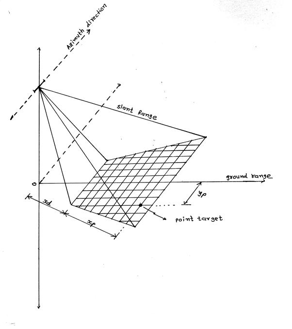
S2.C2.D2

S2.C2.3 POINT TARGET GEOMETRY FOR ASAR

In Figure S2.C2.D3 & in Figure S2.C2.D4 Point Target Geometry for ASAR in Azimuth-Slant Range plane (Top view) and in Range-Altitude plane (Elevation view) is depicted respectively. First Figure S2.C2.D3 tells about the Synthetic Aperture Length, Aperture Time for data collection and total Doppler Bandwidth from the parameters like

· The shortest Slant Range distance between air-craft and point target

· Velocity of air-craft, actual Antenna Length and Wavelength

· Horizontal (Azimuth) Antenna Beam-width q_H

Second Figure S2.C2.D4 tells about the Vertical (Range) Beam-width q_V of the antenna, Antenna Look Angle, distance of the swath from Nadir track and Swath-width.

S2.C2.D3

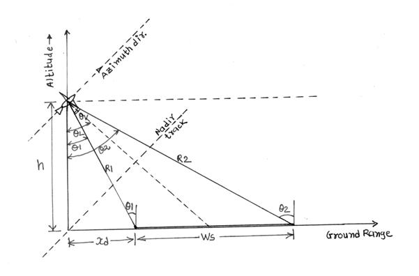
R1 - Minimum Near Slant Range = 8000 m

R2 - Maximum Far Slant Range » 32000 m

q1,q2 – Incidence Angles, q1 » 41.40°, q2 » 78.79°

qv – 3dB Vertical Beam-width, Range Beam-width » 37.38°

qL – Look Angle » 60°

Ws – Swath-width » 25 kms

h – Altitude » 6000 m

xd » 5.29 m

S2.C2.D4

S2.C2.4 DATA COLLECTION, STORAGE & PROCESSING

As such there is no need to have data collection and storage for a point target simulation. LFM (Chirp) data (samples) are generated in MATLAB, which are analogous to a data set (some single column) for a given Range Gate, of actually mapped 2-D data gathered during the observation time. Figure S2.C2.D5 illustratively clears the whole picture of 2-D data organization. Every PRF (Pulse Repetition Frequency) return is stored row wise from near-to-far range and each element (data) in that row corresponds to a single resolution cell in the range direction. The collection of such several PRF returns stacked together forms equal numbers of columns as the number of range gates or range cells in Range direction. Near Range column has a smaller dimension compared to a Far Range column because of different Aperture Time and different Synthetic Aperture Length for different Range Gates. Intersections of all rows and columns give formation of 2D cells, any one of that is identified as i^th range gate in j^th PRF return. Interestingly the data set, a sampled version of a return signal in both range and azimuth directions carry the LFM (Chirp) nature. Of course LFM shape row-wise is obvious, as the transmitted signal is LFM only and there is only a point target to interact with it, but because of Doppler effect the same constant transmitted frequency for all cells in a given column (Range Gate) takes the LFM shape when viewed as a return. This phenomenon called Doppler effect is the result of relative motion between a steady point target on the ground and a moving radar platform on the air-craft.

Now with the clear idea about 2-D data organization, processing is the implementation of various algorithms on a selected data set. Out of two basic types of signal processing (correlation) required for high-resolution ground imaging,

1 Range processing &

2 Azimuth processing, it is assumed to have Range processed data available for further Azimuth processing.

Here the row wise data in 2-D space are assumed to be Range compressed (processed). Azimuth processing is done to improve the Azimuth Resolution of the ground image. Time-Domain (TASP) and Frequency-Domain (FASP) are the two fundamental approaches with different implementation requirements, trade-offs, advantages and limitations generally used for Azimuth Signal Processing. Both approaches for a given point target rely on a same data set (i^th column of n 1-D samples) which is generated by LFM equation in MATLAB workspace.

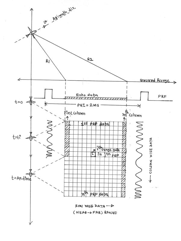
S2.C2.D5

S2.C2.5 END RESULTS

After processing a given data set having LFM shape turns to be a sharp long peak with several side lobes. The amplitude of the peak is mapped with some intensity level to a corresponding pixel on the display monitor representing the characteristic of a point target. Quality of image and ground feature extraction depends on the following two End Results (outcomes) that can be derived from finally processed data set (registered data) having a distinct peak and side lobe nature.

1 Azimuth Resolution

2 ISLR (Integrated Side Lobe Ratio)

Registered data set is quite small in dimension due to moderately small Azimuth Resolution and multi-look processing necessity in practical situations. As shown in Figure S2.C2.D6, to estimate the End Results in effective manner, registered data is interpolated by some suitable factor, and from the magnitude response of the interpolated data, number of samples within 3-dB threshold are calculated. These samples are the spatial 3-dB resolution samples.

Azimuth Resolution is directly proportional to the number of 3-dB resolution samples. Formulation of exact equation for Azimuth Resolution depends on the approach used for processing. It tells about smallest possible ground feature extraction.

ISLR (dB) is the ratio of energy contained in significant side lobes around the peak and the energy within 3-dB of a peak response. ISLR tells about an image quality in terms of inter pixel interference, blurring or the sharpness of extracted features.

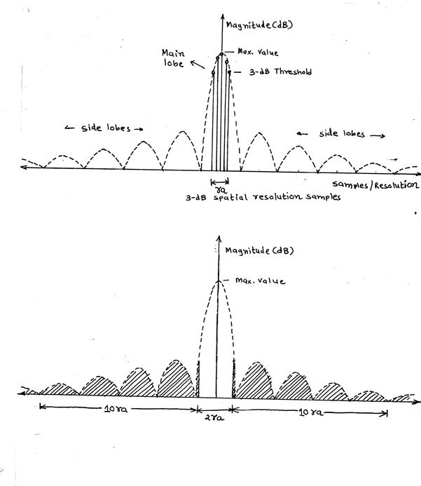
ISLR = Energy of the Shaded Area

Energy of the non Shaded Area

ra = Number of 3dB resolution samples

S2.C2.D6
CHAPTER 3: PARAMETERS & EQUATIONS

For a point target simulation certain system dependant parameters are involved, that characterize the real SAR system. Such standard parameters are listed with their values for both simulation approaches.

There are some flexible variables or parameters, some are common to both approaches others are algorithm selective. As an example Slant Range R is a common variable and has been by default taken as 8000 m.

Very important equations related to SAR signal processing used in both the approaches are also listed below.

S2.C3.1 FIXED- STANDARD PARAMETERS

· Antenna Length: l = 1.3 m, Antenna Width: w = 8 to 9 cm

· Transmitted Signal Wavelength: l = 0.056 m, Frequency: f = 5.3 GHz

· Speed of Air-craft: v =120 m/s

· Pulse Repetition Frequency: PRF = 500 Hz, Antenna Look Angle: q_L » 60°

· Minimum Slant Range: R1 = 8000 m, Maximum Slant Range: R2 = 32000 m

· Air-craft Altitude: h = 6000 m

· Swath-width: Ws = 25000 m

S2.C3.2 IMPORTANT EQUATIONS

· Horizontal Beam-width q_H = l/l, Vertical Beam-width q_V = l/w

· Total Doppler Bandwidth TB = 2.v/l, TB = k. AP_time

· Chirp Rate k = 2.v²/l.R

· Synthetic Length L= l.R/l, L = v.Ts

· Aperture Time AP_time = l.R/l.v = L/v

· Number of Samples Nsamp = AP_time.prf

· Bandwidth selected for required Azimuth Resolution bw, bw = k.t, t = time

· Range Resolution (Slant) dRs = c.t/2, t = Compressed pulse width

· Range Resolution (Ground) dRg = c.t/(2.sinqi), qi = Incident angle

· Azimuth Resolution dAz = v/bw

CHAPTER 4: TIME - DOMAIN APPROACH (TASP)

S2.C4.1 ALGORITHM

Basic block diagram and algorithm flow for Time-Domain approach is shown in Figure S2.C4.B1. Also an acronym guide and program flow supplement is attached in tabular form in Figure S2.C4.T1. The sequence of MATLAB m-files/ Functions is shown in Figure S2.C4.D1. All these three figures are very crucial for further enhancement, modifications and development. Time-Domain approach can be simulated through simulate.m as shown in Figure S2.C4.D1.

The entire processing is in digital domain, hence anywhere the term signal means samples only, even though for better presentation it can be plotted in continuous form in MATLAB figures at several stages during simulation.

	S2.C4.D1

S2.C4.B1

Acronym and Program Flow Supplement for Time-Domain Approach

Block Acronym	Block Name	Description	Input to the Block	Output of the Block
LFM	Linear Frequency Modulation	Generates an Ideal Input Chirp Signal	Runtime? R	yo
GN	Gaussian Noise	Generates White Gaussian Noise of Specified Power	Runtime? Noise pset	g_noise1 or g_noise
A	Addition	Adds Ideal Input Chirp with White Gaussian Noise	yo g_noise 1 or g_noise	y
PF	Pre-Filter	Selects the required bw from total Doppler bw based on number of Looks	y	c
CD5	Decimate by 5	Decimates the Pre-filtered signal by 5	c	cd
LF/LFi	Look Filtering	Separates desired number of Looks by filtering Pre-filtered & decimated signal	cd--cd1,cd2	lki
DC3i	Decimate by 3	Each look signal is again decimated by 3	lki	lkdi
MFi	Match Filtering	Look filtered & decimated i/p signals are convoluted with Reference Function	lkdi	mfoi
Di	Detection	Peak responses after match filtering are converted to magnitude responses without phase information	mfoi	dmfoi
RG	Registration	Registers or integrates the detected peaks at different times by non-coherent averaging	dmfoi	rg
EST3dB	3dB Estimation	Estimates number of samples with in 3-dB of maximum Registered output Peak.	rg	ra
Outcome1	Outcome 1	Presents Azimuth Resolution as the First Image Quality Predictor	ra	Azres
Outcome2	Outcome 2	Presents ISLR as the Second Image Quality Predictor	ra	ISLR

S2.C4.T1

S2.C4.2 BLOCKWISE DESCRIPTION

2.1. Block LFM represents the simulated version of received return in azimuth direction for a given range over a defined Aperture Time with LFM/Chirp equation as below

yo = exp (j.p.k.t²) .....................................................….(2.4.1)

Here yo is an ideal Chirp without any noise effect.

2.2. Block GN generates Additive White Gaussian Noise. It is possible to generate Real as well Complex noise with desired power level of 0.5, 1, 2 or 5 times the complex input signal power yo, which has a unit complex power, obvious from equation 2.4.1. Real noise is denoted by g_noise1 and Complex noise is by g_noise.

2.3. Block A presents the point-to-point addition of input Chirp yo and Gaussian noise g_noise1 or g_noise. It makes an ideal Chirp noisy and offers a better model of truly received return as

y = yo+0 or y = yo+g_noise1 or y = yo+g_noise...........(2.4.2)

If the inserted noise power is zero then y has the same power as yo because the power of y is an addition of power of yo (i.e. 1) and power of Gaussian noise.

2.4. Block PF represents a Pre-filter. The spectrum of input Chirp y is quite large and has a total Doppler bandwidth

TB = 2.v/l ...............................................…………….…(2.4.3)

For any moderate Azimuth Resolution we need only a small portion of this total Doppler bandwith as per

dAz = v/bw Þ bw = v/dAz...............................………………..(2.4.4)

But the inherent problem of multiplicative speckle noise associated with Active Microwave Remote Sensing forces to go for multi-look processing overhead. Hence minimum bandwidth for multi-look processing is number of look times the bandwidth (bw) calculated in equation 2.4.4. The job of Pre-filter is to separate out the required bandwidth portion of the whole Doppler spectrum for multi-look processing.

There are various ways of Pre-filter design. In this application Pre-filter is designed as a Low Pass FIR Filter with different windowing option, and with Actual and Custom Tap Lengths. Parameters needed for a low pass FIR filter design are passband and stopband cutoff frequencies, amount of allowable ripple and a sampling rate. The stringent requirement of minimum side lobe levels with less broadening for a given custom tap length finally ends up with a choice of Kaiser window. End Results of the algorithm implementation or Image quality predictors depend on the tightness or the looseness of a Pre-filter. Implementation of a Pre-filter in Time-Domain is the convolution of input Chirp y and selected window co-efficients, results in a filtered signal c for further processing.

2.5. Block DC5 decimates a Pre-filtered signal c by an integer factor 5 to simulate the need of data reduction for Real-time processing without much adverse effect on the quality of final image. Decimated signal cd is, now with a data size and sampling frequency reduced by an amount equal to the same integer factor (i.e. 5 here).

2.6 Block LE/LEi means Look Extraction or Look Filtering. The decimated signal contains a bandwidth more than the required for a single look. Look Filtering helps in segregation of several looks for independent and simultaneous processing, and speckle reduction. There are two ways for Look Filtering,

1 Design a Low Pass Filter with a fixed spectrum, and shift the input signal spectrum as required by exponential multiplication in time.

2 Transformation of LPF to BPF, shifting of spectral response of BPF as required and keeping input signal spectrum stationary.

The first method is explored here in view to adopt the same design methodology of Pre-filter with only changes in supplied parameters for Look Filter. Analogous to shifting of input spectrum in frequency is multiplication in time by an exponential factor. Depending on look bandwidth and number of multi-looks, it is at least marginally convenient to go for first method. Here the tightness or the looseness of the filter contributes a lot to the computation as a result of precise bandwidth extraction for each look. Amount of variations in shifting of input signal spectrum is also a significant factor.

Original input- decimated signal cd and its exponential multiplied versions cdi (equation 2.4.5) as an input to Look Filter produce look filtered output signals lki by the same convolution approach.

cdi= cd. exp( ± j.2.p.f0.t).........…………....................….(2.4.5)

2.7 Block DC3i again represents decimation of Look Filtered signal lki by 3; picking up every third sample of the sequence only. Output signals after DC3i are lkdi.

2.8 Block MFi is a Match Filter bank. Corresponding to each Look Filtered signal there is one Match Filter. Match Filter represents a pre-determined Reference Function similar to input Chirp but smaller in length. Match Filtering is the process of correlation between Reference Function and Look Filtered signals lkdi. It gives sharp peak response mfoi at different time indices for different looks.

2.9 Block Di is a Detection process. Peak responses after Match Filtering are complex valued. Detection means conversion of such complex valued signals to their magnitude (absolute) form, suitable for an image display. Information about phase is lost at this point. Detected outputs are dmfoi.

2.10 Block RG models Registration/Integration process of all detected looks, means the absolute peak responses at different time indices are non-coherently added and averaged. It reduces speckle noise and gives better image quality. Registered output is rg.

2.11 Outcomes: Determination of End Results/Outcomes is subsequent to the registration process. Registered output rg is small in size due to decimation by a factor of 15 during the whole process and hence it is interpolated at least by a factor of 15 for better 3-dB resolution samples estimation. Higher interpolation factors give stable estimate. With the help of 3-dB resolution samples estimate, sharpness of a registered peak response is judged in terms of Azimuth Resolution and side lobe levels & spread in terms of ISLR.

Outcome1: Azimuth Resolution : It is the first End Result after a long, complex and very involved processing chain. It should be as minimum as possible for the extraction of very minute ground features with due clarity. Azimuth Resolution in Time-Domain approach is summarized as...

Azimuth Resolution (dAz) µ v v: Velocity of Air-craft

µ 1/PRF PRF: Pulse Repetition Frequency

Outcome2: ISLR( Integrated Side Lobe Ratio) : It is the second End Result, It should be as high as possible in ( - dB scale). It can be summarized as...

ISLR = Total Energy content out of 3-dB Main Lobe & in all significant Side Lobes

Energy within 3-dB Main Lobe

S2.C4.3 RESULTS

At the end, for Time-Domain Azimuth Signal Processing Approach (TASP), several important design/simulation parameter selections, effect of parameter variations and effect of noise on the End Results are shown below as a representative set.

· System Parameters : ( Side Looking Stripmap SAR)

Velocity of Air-craft- 120 m/s

Actual Antenna Length- 1.3 m, Antenna Width- 8 to9 cm

Air-craft Altitude- 6000 m

Center Wavelength- 0.056 m

· Simulation case study :

Slant Range(R) = 8000 m, Chirp Rate (k) = 63.60 Hz/s,

Aperture Time (AP_time) =2.9028 sec

Number of Samples of i/p Chirp (No_samp) = 1451,

Synthetic Aperture Length (L) = 348.33 m,

Reference Function Length (Ref_len) = 13.62

Signal Power = 1, Noise Power (Real/Complex)= Variable (0,0.5,1,2...100)

Interpolation Factor = 15

3.1 Comprehensive summary of selected Parameter variations for a Point Target at different Slant Range (Near®Far)

S2.C4.T3.1

Parameters ¯		Slant Range R (m) from 6000m Altitude
		8000	10,000	15,000	20,000	25,000	30,000	32,000
AP_time(sec)		2.9028	3.6284	5.4427	7.2569	9.0711	10.8853	11.6110
L(m)		348.33	435.41	653.12	870.82	1088.50	1306.20	1393.30
No_samp		1451	1815	2712	3629	4537	5443	5807
K(Hz/sec)		63.60	50.88	33.92	25.44	20.35	16.96	15.90
Rf_len		13.62	17.03	25.55	34.06	42.58	51.10	54.50
Det_size		121	149	218	286	357	425	454
Det_pos	Aft	47	57	84	109	136	162	173
	Center	61	75	109	143	179	213	227
	Fore	74	92	135	177	221	264	282
Det_mag	Aft	10.58	11.12	19.60	27.15	33.21	33.47	44.25
	Center	11.12	12.93	21.38	31.31	38.72	41.31	41.74
	Fore	9.88	11.71	20.17	26.76	30.55	38.20	44.25
Rg_size		153	189	274	360	447	533	568
Rg_pos		74	92	135	177	221	264	282
Rg_mag(NW)		10.53	11.92	20.38	28.41	34.16	37.66	43.41
Rg_mag(HW)		7.53	8.89	14.72	20.27	25.02	28.14	31.57
ISLR (dB) (NW)		-9.87	-11.05	-10.32	-9.93	-10.85	-13.24	-11.31
Azres (m) (NW)		4.80	5.52	4.80	4.56	4.80	5.28	5.04
ISLR (dB) (HW)		-17.80	-17.30	-18.17	-18.54	-18.57	-18.97	-19.48
Azres (m) (HW)		6.00	5.52	5.76	5.52	5.76	5.52	5.76

3.2 Actual Tap Length of Low Pass FIR Filter with 3 different windows

S2.C4.T3.2.1 Pre-filter

fpb	fsb	Passband/stopband Ripple rp/rs (dB)	fs	Actual Tap Length
				Boxcar Nbcar	Hamming Nham	Kaiser Nkais
39	61	40	500	21	79	53
39	50	40	500	42	158	103
39	45	40	500	77	290	187
39	40	40	500	460	1735	1117
39	61	20	500	21	79	21
39	61	30	500	21	79	37
39	61	50	500	21	79	69
39	61	60	500	21	79	85

S2.C4.T3.2.2 Look Filter

fpb	fsb	Passband/Stopband Ripple rp/rs (dB)	fs	Actual Tap Length
				Boxcar Nbcar	Hamming Nham	Kaiser Nkais
13	20.33	40	100	13	48	33
13	20	40	100	14	50	33
13	15	40	100	47	174	113
13	14	40	100	92	347	225
13	20.33	30	100	13	48	23
13	20.33	50	100	13	48	41
13	20.33	60	100	13	48	51

fpb: Passband cutoff frequency rp: Passband Ripple in dB

fsb: Stopband cutoff frequency rs: Stopband Ripple in dB

fs: Sampling Rate

Nbcar: Boxcar Window Tap Length

Nham: Hamming Window Tap Length

Nkais: Kaiser Window Tap Length

3.3 Effect of different window weighting without noise

S2.C4.T3.3.1 Custom Tap Length Filtering

S2.C4.T3.3.1.1

LPF type	Fpb	Fsb	Stopband Ripple Attenuation(dB)	Fs	Window Type	Tap Length
Pre-Filter	39	61	40	500	Kaiser	31
Look Filter	13	20.33	40	100	Kaiser	31

S2.C4.T3.3.1.2 Noise Power: 0

Reference Function Weighting	3-dB resolution samples (ra)	Azimuth Resolution (Azres) m	ISLR (dB)
Boxcar	20	4.80	-9.87
Hamming	25	6.00	-17.80
Hanning	27	6.48	-21.65
Blackman	33	7.92	-20.20
Dolf-Chebyshev	28	6.72	-21.07
Kaiser	27	6.48	-21.66

S2.C4.T3.3.2 Actual Tap Length Filtering

S2.C4.T3.3.2.1

LPF type	Fpb	Fsb	Stopband Ripple Attenuation(dB)	Fs	Window Type	Tap Length
Pre-Filter	39	61	40	500	Kaiser	Actual
Look Filter	13	20.33	40	100	Kaiser	Actual

S2.C4.T3.3.2.2 Noise Power: 0

Reference Function Weighting	3-dB resolution samples (ra)	Azimuth Resolution (Azres) m	ISLR (dB)
Boxcar	21	5.04	-10.35
Hamming	25	6.00	-18.09
Hanning	27	6.48	-21.84
Blackman	33	7.92	-20.14
Dolf-Chebyshev	29	6.96	-22.31
Kaiser	27	6.48	-21.85

3.4 Comparison between Custom/Actual Tap Length Filtering without noise

S2.C4.T3.4.1 Filtering with Custom Tap Length without Noise

S2.C4.T3.4.1.1

LPF type	Fpb	Fsb	Stopband Ripple Attenuation(dB)	Fs	Window Type	Tap Length
Pre-Filter	39	61	40	500	Kaiser	31
Look Filter	13	20.33	40	100	Kaiser	31

S2.C4.T3.4.1.2 Noise Power: 0

Reference Function Weighting	3-dB resolution samples (ra)	Azimuth Resolution (Azres) m	ISLR (dB)
Boxcar	20	4.80	-9.87
Hamming	25	6.00	-17.80
Kaiser	27	6.48	-21.81

S2.C4.T3.4.2 Filtering with Actual Tap Length without Noise

S2.C4.T3.4.2.1

LPF type	Fpb	Fsb	Stopband Ripple Attenuation(dB)	Fs	Window Type	Tap Length
Pre-Filter	39	61	40	500	Kaiser	Actual
Look Filter	13	20.33	40	100	Kaiser	Actual

S2.C4.T3.4.2.2 Noise Power: 0

Reference Function Weighting	3-dB resolution samples (ra)	Azimuth Resolution (Azres) m	ISLR (dB)
Boxcar	21	5.04	-10.35
Hamming	25	6.00	-18.09
Kaiser	27	6.48	-21.85

3.5 Filtering with Custom Tap Length in noise

S2.C4.T3.5.1

LPF type	Fpb	Fsb	Stopband Ripple Attenuation(dB)	Fs	Window Type	Tap Length
Pre-Filter	39	61	40	500	Kaiser	31
Look Filter	13	20.33	40	100	Kaiser	31

S2.C4.T3.5.2 Real Noise Power: 1 (case 1)

Reference Function Weighting	3-dB resolution samples (ra)	Azimuth Resolution (Azres) m	ISLR (dB)
Boxcar	21	5.04	-7.22
Hamming	25	6.00	-8.89
Kaiser	28	6.72	-9.23

S2.C4.T3.5.3 Real Noise Power: 1 (case 2)

Reference Function Weighting	3-dB resolution samples (ra)	Azimuth Resolution (Azres) m	ISLR (dB)
Boxcar	20	4.80	-7.11
Hamming	24	5.76	-9.77
Kaiser	26	6.24	-9.95

S2.C4.T3.5.4 Complex Noise Power: 1 (case 1)

Reference Function Weighting	3-dB resolution samples (ra)	Azimuth Resolution (Azres) m	ISLR (dB)
Boxcar	21	5.04	-6.41
Hamming	25	6.00	-7.50
Kaiser	27	6.48	-7.57

S2.C4.T3.5.5 Complex Noise Power: 1 (case 2)

Reference Function Weighting	3-dB resolution samples (ra)	Azimuth Resolution (Azres) m	ISLR (dB)
Boxcar	20	4.80	-6.14
Hamming	24	5.76	-7.86
Kaiser	26	6.24	-7.88

S2.C4.T3.5.6 Real Noise Power: 2 (case 1)

Reference Function Weighting	3-dB resolution samples (ra)	Azimuth Resolution (Azres) m	ISLR (dB)
Boxcar	21	5.04	-4.65
Hamming	25	6.00	-5.02
Kaiser	27	6.48	-4.87

S2.C4.T3.5.7 Real Noise Power: 2 (case 2)

Reference Function Weighting	3-dB resolution samples (ra)	Azimuth Resolution (Azres) m	ISLR (dB)
Boxcar	21	5.04	-5.79
Hamming	25	6.00	-6.67
Kaiser	27	6.48	-6.26

S2.C4.T3.5.8 Complex Noise Power: 2 (case 1)

Reference Function Weighting	3-dB resolution samples (ra)	Azimuth Resolution (Azres) m	ISLR (dB)
Boxcar	22	5.28	-4.73
Hamming	26	6.24	-5.98
Kaiser	28	6.72	-6.04

S2.C4.T3.5.9 Complex Noise Power: 2 (case 2)

Reference Function Weighting	3-dB resolution samples (ra)	Azimuth Resolution (Azres) m	ISLR (dB)
Boxcar	21	5.04	-5.45
Hamming	25	6.00	-7.10
Kaiser	27	6.48	-7.14

S2.C4.T3.5.10 Real Noise Power: 10 (case 1)

Reference Function Weighting	3-dB resolution samples (ra)	Azimuth Resolution (Azres) m	ISLR (dB)
Boxcar	25	6.00	-0.70
Hamming	28	6.72	-0.61

S2.C4.T3.5.11 Real Noise Power: 10 (case 2)

Reference Function Weighting	3-dB resolution samples (ra)	Azimuth Resolution (Azres) m	ISLR (dB)
Boxcar	21	5.04	-0.03
Hamming	24	5.76	0.19

S2.C4.T3.5.12 Complex Noise Power: 10 (case 1)

Reference Function Weighting	3-dB resolution samples (ra)	Azimuth Resolution (Azres) m	ISLR (dB)
Boxcar	24	5.76	0.31
Hamming	29	6.96	0.08

S2.C4.T3.5.13 Complex Noise Power: 10 (case 2)

Reference Function Weighting	3-dB resolution samples (ra)	Azimuth Resolution (Azres) m	ISLR (dB)
Boxcar	27	6.48	3.78
Hamming	30	7.20	3.52

3.6 Filtering with Actual Tap Length in noise

S2.C4.T3.6.1

LPF type	Fpb	Fsb	Stopband Ripple Attenuation(dB)	Fs	Window Type	Tap Length
Pre-Filter	39	61	40	500	Kaiser	Actual
Look Filter	13	20.33	40	100	Kaiser	Actual

S2.C4.T3.6.2 Real Noise Power: 1 (case 1)

Reference Function Weighting	3-dB resolution samples (ra)	Azimuth Resolution (Azres) m	ISLR (dB)
Boxcar	21	5.04	-7.49
Hamming	25	6.00	-9.20
Kaiser	27	6.48	-9.33

S2.C4.T3.6.3 Real Noise Power: 1 (case 2)

Reference Function Weighting	3-dB resolution samples (ra)	Azimuth Resolution (Azres) m	ISLR (dB)
Boxcar	21	5.04	-7.13
Hamming	25	6.00	-9.54
Kaiser	27	6.48	-9.89

S2.C4.T3.6.4 Complex Noise Power: 1 (case 1)

Reference Function Weighting	3-dB resolution samples (ra)	Azimuth Resolution (Azres) m	ISLR (dB)
Boxcar	20	4.80	-5.70
Hamming	24	5.76	-8.11
Kaiser	26	6.24	-8.32

S2.C4.T3.6.5 Complex Noise Power: 1 (case 2)

Reference Function Weighting	3-dB resolution samples (ra)	Azimuth Resolution (Azres) m	ISLR (dB)
Boxcar	21	5.04	-7.45
Hamming	25	6.00	-9.03
Kaiser	27	6.48	-9.05

S2.C4.4 INTERPRETATIONS

Based on the representative tabularized result set (S2.C4.3) derived from Time-Domain Azimuth Signal Processing Approach (TASP), important comments/interpretations are deduced as below.

Ø Single shot review of different parameter variations is presented in Table of 3.1. The important points derived from the table are as below:

· Synthetic Aperture Length (width of footprint) increases from near-to-far range but Azimuth Resolution remains almost constant.

· Peaks of registered output appear at different positions, for different-range point targets, shows correct distance estimation ability of TASP.

· The magnitude of registered peak increases from near-to-far range because of successive long correlation through Match Filtering, which is suggestive for the need of Radiometric Correction.

· ISLR without/with weighting remains almost constant throughout the swath width. Weighted Match Filtering has quite vivid improvement in ISLR, as well as an important role in maintaining baseline Azimuth Resolution in ideal or upto equal signal power noise conditions.

Ø Tightness (small transition band) of FIR LPF increases its tap length, and in turn computation overhead (convolution). (Tables of 3.2)

Ø For Pre-filter or Look Filter, Kaiser window is the best choice as it gives reasonably less tap length than Hamming window and better adjustable ripple reduction. Although it has more broadening compared to Hamming window, smooth roll-off acceptance for both filters makes Kaiser window as an optimum choice. Boxcar window with the least broadening, minimum tap length is not suitable as it has the highest side lobe ripples. (Tables of 3.2)

Ø As Pre-filter helps in additional noise cut-off, smooth roll-off has no significant adverse effect on End Results, but the tap length will drastically reduce. Even custom tap length of 31 compared to actual 53 is good enough. (Table S2.C4.T3.2.1)

Ø Reasonable tightness of Look Filter is justified, as it is crucial for processing bandwidth extraction. Custom length of 31 tap; almost equal to actual length of 33, for 26Hz processing bandwidth requirement is justified as per Table S2.C4.T3.2.2.

Ø For Pre-filter/Look Filter with actual tap length has marginally but improved ISLR compared to custom tap length. In both cases Azimuth Resolution is almost same except Boxcar weighting. (Tables of 3.3)

Ø Hamming (a=0.7) window weighting is an optimum choice with Azimuth Resolution and ISLR trade-off, without noise (AWGN). (Tables of 3.3)

Ø Tightening of Pre-filter/Look Filter or actual tap length filtering, Match Filtering with no weighting of Reference Function broadens the peak response, hence poor Azimuth Resolution with very small improvement in ISLR. (Tables of 3.4)

Ø Match Filtering with Boxcar weighting of Reference Function has the best peak response of registered output and the minimum dimension (best) of Azimuth Resolution at the cost of poorer (Minimum - in absolute magnitude form) ISLR of registered peak output. (Tables of 3.3 and 3.4)

Ø Match Filtering with different window weighting of Reference Function has improved ISLR but blunt (broadened) registered peak response, hence large dimension (poor) of Azimuth Resolution. (Tables of 3.3 and 3.4)

Ø Under the condition of noisy received return, AWGN of equal signal power (i.e. 1) has significant effect on ISLR deterioration but Azimuth Resolution is almost unaffected. For AWGN of double the signal power (i.e. 1), ISLR has even more deterioration and Azimuth Resolution just starts aggravating. Under very large power (e.g. 10 times or more than signal power) AWGN, ISLR approaches zero and then moves towards positive and Azimuth Resolution gets even poorer. Although both ISLR and Azimuth Resolution depend on the AWGN sample distribution, which is time variant. (Tables of 3.5 and 3.6)

Ø As far as ISLR is concerned, Hamming weighting is significant upto equal signal power AWGN only. As noise power increases, distinction between with Boxcar weighted and Hamming weighted ISLR diminishes (Tables of 3.5 and 3.6)

Ø For the same amount of AWGN power, complex noise affects ISLR more than real noise. Both types of noise almost equally affect the Azimuth Resolution, which is more or less constant and same as without any noise under the equal signal power noise or moderately high noise power conditions. (Tables of 3.5 and 3.6)

Ø Actual tap length Pre-filtering/Look Filtering has marginally better ISLR in noisy environment compared to custom tap length (31) filtering but Azimuth Resolution on average remains same, separately in both types of noises, and with three types of weightings. (Tables of 3.5 and 3.6)

Ø Slant Range Resolution is constant for the entire Swath-width and is determined by range compressed pulse width. Ground Range Resolution is a function of incident angle at that Slant Range and it deteriorates from near-to-far range. (Equations of S2.C3.2)

CHAPTER 5: FREQUENCY - DOMAIN APPROACH (FASP)

S2.C5.1 ALGORITHM

Implementation of Frequency-Domain approach with two possible options is highlighted in Figure S2.C5.B1 (Frequency Weighting FW-FASP) & in S2.C5.B2 (Time Weighting TW-FASP). An Acronym and Program Flow Supplement as shown in Figure S2.C5.T1 gives overview of block wise description, input/output signals and the End Results for both algorithms. Here because of large time-bandwidth LFM signal, both algorithms: weighting in Time & weighting in Frequency are explored. For Match Filtering look-to-look matching is presumed for both cases having the advantage of same position detection-registration. Even the other carried out approach of only central-look matching gives almost same End Results but the different position detection makes registration process more complex.

Both algorithms can be tested, simulated and further enhanced depending on future requirements with the M-files fw.m for Frequency Weighting and tw.m for Time Weighting.

The most important aspect of Frequency-Domain approach is Block-Processing, different than sample-by-sample convolution method in Time-Domain approach. Of course the same kind of correlation analogous to convolution in time is carried out as a multiplication in Frequency-Domain. Chirp signal generation, AWGN addition and End Results (Outcomes) determination methods still remain same as Time-Domain approach. Transformation of Time to Frequency is done through FFT for processing, and inverse transformation from Frequency to Time is done through IFFT for outcome analysis. Referring to chapter S2.C4 and Table S2.C4.T3.1 of Time-Domain approach, for full swath or narrow swath, far-range imaging using Frequency-Domain approach, 8K FFT is must. Choice of number of IFFT points for Frequency to Time transformation depends on the desired Azimuth Resolution as per Table S2.C5.T2. There is no Pre-filtering in both Time Weighted Frequency-Domain Azimuth Signal Processing (TW-FASP) or in Frequency Weighted Frequency-Domain Azimuth Signal Processing Approach (FW-FASP).

S2.C5.B1

S2.C5.B2

Acronym and Program Flow Supplement for Frequency-Domain Approach

Frequency Weighting

Block Acronym	Block Name	Description	Input to the Block	Output of the Block	Detailed Flow Diagram
LFM	Linear Frequency Modulation	Generates an Ideal Input Chirp Signal	Runtime R	yo	S2.C5.F1
GN	Gaussian Noise	Generates White Gaussian Noise of Specified Power	Runtime noise pset	g_noise1 or g_noise	S2.C5.F2
A	Addition	Adds Ideal Input Chirp & White Gaussian Noise	yo, g_noise 1 or g_noise	y	S2.C5.F3
T2F1	Time to Frequency	Transforms Noisy Chirp from Time to Frequency-Domain by 8K FFT	y	yf	S2.C5.F4
RF	Reference Function	Generates Reference (Match) Function similar but Complex Conjugate of Ideal Input Chirp	Derived from Runtime Input to LFM	mfun	S2.C5.F5
T2F2	Time to Frequency	Transforms Reference Function from Time to Frequency-Domain by 8K FFT	mfun	mfunf	S2.C5.F6
WCW	Weighting Coeff. Window	Selects Weighting Co-eff. Window of suitable length from a given set of Window Types.	Derived from Processing bw, prf and FFT size 8K.	mtwgtd	S2.C5.F7
WF	Weighting Frame	Creates entire 8K Weighting Frame by repetitive placing of Weighting Window	mtwgtd	wframe	S2.C5.F8
M1	Multiply	Multiplies 8K FFT of Reference Function and 8K Weighting Frame	mfunf, wframe	Full mulw	S2.C5.F9
M2	Multiply	Multiplies Weighted 8K FFT of Reference Function and 8K FFT of Input Chirp	fullmulw, yf	waves	S2.C5.F10
LE/LEi	Look Extraction	Extracts Single/Multiple Look/Looks of specified processing bw in terms of Frequency-Domain Sample Points	waves	mul0, mul(i,:)	S2.C5.F11
F2Ti	Frequency to Time	Transforms selected Look/Looks to its equivalent Time-Domain by IFFT	mul0, mul(i,:)	det0c, detc(i,:)	S2.C5.F12
Di	Detection	Computes the Magnitude of Complex Freq. To Time Transformed Look output	det0c, detc(i,:)	det0, det(i,:)	S2.C5.F13
RG	Registration	Registers or Integrates the Single/Multiple Detected output by Non-coherent Averaging	det0, det(i,:)	rg	S2.C5.F14
EST3dB	3dB Estimation	Estimates number of samples with in 3-dB of max. Registered output.	rg	rad	S2.C5.F15
Outcome 1	Outcome 1	Presents Azimuth Resolution as the First Image Quality Predictor	rad	Azres	S2.C5.F16
Outcome 2	Outcome 2	Presents ISLR as the Second Image Quality Predictor	rad	ISLR	S2.C5.F17

S2.C5.T1

Some Important Equations and Sample Calculation Example for FW-FASP

· Azimuth Resolution (Azres or dAz) = v/bw

Þ bw = v/dAz

· Bandwidth represented by each sample of

8K correlated frame (sampf) = prf/8K

= 500/8192 = 0.061

· Total Doppler Bandwidth (TB) = 2.v/l » 184 Hz

Þ Effective samples for processing = 184/0.061

» 3017 (3016)

Lets take the case of Azimuth Resolution “better than 6m”

Take bw = 26 hz Þ Expected dAz = 120/26 = 4.61 m (< 6 m)

Number of samples for IDFT = bw/sampf = 26/0.061 » 427

Number of samples for IFFT = Next power of 2 of (427) = 512

Number of Max. looks for IDFT= Truncated integer of [(3016/2)/427 *2] = 7

Number of Max. looks for IFFT= Truncated integer of [(3016/2)/512 *2] = 5

Desired Azimuth Resolution (m)	Required Processing Bandwidth (Hz)	Number of IDFT Points/look	Number of IFFT Points/look	Max. Possible Looks with IDFT	Max. Possible Looks with IFFT
10	12	197	256	41 à15	32 à 11
6	20	328	512	24 à 9	16 à 5
3	40	656	1024	12 à 4	8 à 2
1	120	1968	2048	4 à1	4 à 1
Better than 6m	26	427	512	19 à 7	16 à 5
Better than 6m	31.25	512	512	16 à 5	16 à 5

S2.C5.T2

S2.C5.2 BLOCKWISE DESCRIPTION

Referring to block diagrams S2.C5.B1 and S2.C5.B2, several blocks are similar to Time-Domain approach like LFM, GN, A, RG, Outcome1 and Outcome2. In this approach decimation is not carried out, hence processing on large data set is involved. The core processing is done in Frequency-Domain so it is identified as FASP. Generalized functional description of important blocks for both TW-FASP and FW-FASP is summarized as follow. Detailed block wise program flow for FW-FASP is documented in flow charts S2.C5.F1 to S2.C5.F17.

2.1 Block T2F1 transforms input Chirp samples of Time-Domain to Frequency-Domain by 8K FFT. The FFT size of 8K is justified because of the largest data set for far-range (32000m) is above 5000 samples. If the data set is less than 8K, trailing points are padded with zeros to make the data set size uniform.

2.2 Block RF generates Reference (Match) Function, similar but complex conjugate of input LFM signal. The data size is also same as input Chirp signal.

2.3 Block T2F2 takes 8K FFT of Reference Function and transforms it in Frequency-Domain so that the essence of the whole algorithm i.e. correlation, can be done as a multiplication in Frequency-Domain.

2.4 Block WC generates pre-determined points of Weighting Window Coefficient. Number of weighting window points is different for both TW-FASP and FW-FASP.

For TW-FASP: Number of points = No_samp*bw/TB…………………….(2.5.1)

For FW-FASP: Number of points = bw/(prf/8192) .…………….…………(2.5.2)

These coefficients are responsible for better ISLR at the cost of broadened main lobe peak response. From a large set of Windows, generally Hamming or Kaiser Window is selected.

2.5 Block WF generates entire Weighting Frame by repeating weighting window coefficient points over 8K size for FW-FASP and over Reference Function size for TW-FASP. This Weighting Frame can be thought of as a shaping mask. For TW-FASP, shaping of Reference Function is done in time whereas for FW-FASP, shaping is applied on a Frequency-Domain version of Reference Function.

2.6 Block M1 performs above-mentioned shaping of Reference Function. The difference in TW-FASP and FW-FASP is just the altered positions of blocks T2F2 & M1 as per block diagrams S2.C5.B1 and S2.C5.B2.

2.7 Block M2 multiplies the weighted (shaped) Reference Function and input Chirp in Frequency-Domain. This block corresponds to correlation as a multiplication in Frequency-Domain. From this block onwards both FASP algorithms are similar.

2.8 Block LE/LEi determines the selection of desired bandwidth (bw) for a given Azimuth Resolution by picking up a set of weighted points (a look) from a correlated frame (output from Block M2). Here multi-look processing is possible with an option LEi by picking up same number of required points but from different portions (looks) of correlated 8K frame. This multi-look processing gives better results in the presence of speckle noise and AWGN.

2.9 Block F2Ti again transforms back the selected looks (by LE/LEi) to Time-Domain by taking IDFT/IFFT on the extracted look/looks. Depending on the processing bw, number of points of extracted look may vary and it may not be in power of 2 size, for such cases IDFT is used or data is padded with zeros to make it next power of 2 size. This block gives complex peak response in time.

2.10 Block Di is represents detection and it gives absolute magnitude of the complex peak response. For single look, there is only one peak response so the detection or registration is same. For multi-look processing, there are i peak responses but they all are positioned at a same mark on x-axis because of look-to-look matching.

2.11 Block RG, Outcome1 and Outcome2 are identical as Time-Domain approach (TASP).

S2.C5.F1

S2.C5.F2

S2.C5.F3

S2.C5.F4

S2.C5.F5

S2.C5.F6

S2.C5.F7

S2.C5.F8

S2.C5.F9, S2.C5.F10

S2.C5.F11

S2.C5.F12

S2.C5.F13

S2.C5.F14

S2.C5.F15

S2.C5.F16

S2.C5.F17

S2.C5.3 RESULTS

End Results i.e.

1 Azimuth Resolution &

2 ISLR,

for both TW-FASP & FW-FASP algorithms are tabularized as a representative set with various parameters like, processing bandwidths (bw), number of IDFT/IFFT points, Weighting Window, amount of AWGN power etc. to highlight the following issues.

If nothing is mentioned with the table, it is assumed that there is no noise, no weighting and central look registration with Interpolation factor =15.

· Selected bw =20/26/31.25 Hz with both IDFT and IFFT, with different weights for both TW-FASP & FW-FASP.

· 256,1024,2048 points single look IFFT with different weights for FW-FASP.

· 512 points/31.25 Hz with single/3 looks, with different weights in ideal as well as in noisy environment.

· Effect of interpolation factor.

3.1 Processing bw = 20/26/31.25 for TW-FASP

S2.C5.T3.1.1 bw=20, central look, TW-FASP

Reference Function Weighting	Peak (dB)	3-dB resolution samples (ra)	Azimuth Resolution (Azres) m	ISLR (dB)
Boxcar	71.84	13	5.20	-17.60
Hamming	68.72	15	6.00	-19.35
Kaiser	68.05	17	6.80	-18.19
Hanning	65.99	21	8.40	-19.37
Blackman	64.37	24	9.60	-18.85
Dolf-Chebyshev	67.19	18	7.20	-18.22

S2.C5.T3.1.2 bw=26, central look, TW-FASP

Reference Function Weighting	Peak (dB)	3-dB resolution samples (ra)	Azimuth Resolution (Azres) m	ISLR (dB)
Boxcar	69.62	21	6.46	-8.81
Hamming	67.70	19	5.84	-14.83
Kaiser	67.43	19	5.84	-16.36
Hanning	65.80	22	6.76	-18.62
Blackman	64.30	26	8.00	-21.00
Dolf-Chebyshev	66.72	20	6.15	-18.41

S2.C5.T3.1.3 bw=31.25, central look, TW-FASP

Reference Function Weighting	Peak (dB)	3-dB resolution samples (ra)	Azimuth Resolution (Azres) m	ISLR (dB)
Boxcar	69.83	19	4.86	-8.52
Hamming	67.84	18	4.60	-14.39
Kaiser	67.53	19	4.86	-17.86
Hanning	65.83	21	5.37	-18.86
Blackman	64.34	25	6.40	-20.43
Dolf-Chebyshev	66.83	20	5.12	-19.53

3.2 Processing bw = 20/26/31.25 for FW-FASP

S2.C5.T3.2.1 bw=20, FW-FASP

Ref. Function Weighting	328 points-IDFT				512 points -IFFT (Zero padded)
	Peak	ra	Azres	ISLR	Peak	ra	Azres	ISLR
Boxcar	71.84	13	5.19	-17.60	68.14	20	5.12	-10.33
Hamming	68.75	15	5.99	-19.47	64.96	24	6.14	-16.59
Kaiser	68.09	17	6.79	-18.28	64.27	27	6.91	-20.48

S2.C5.T3.2.2 bw=26, FW-FASP

Ref. Function Weighting	427 points-IDFT				512 points -IFFT (Zero padded)
	Peak	ra	Azres	ISLR	Peak	ra	Azres	ISLR
Boxcar	69.62	21	6.46	-8.81	69.22	20	5.12	-11.27
Hamming	67.81	19	5.84	-15.35	66.95	19	4.86	-18.11
Kaiser	67.55	19	5.84	-19.45	66.42	21	5.37	-21.15

S2.C5.T3.2.3 bw=26, 3-looks, FW-FASP

Ref. Function Weighting	427 points-IDFT				512 points -IFFT (Zero padded)
	Peak	ra	Azres	ISLR	Peak	ra	Azres	ISLR
Boxcar	69.62	21	6.46	-8.81	67.67	18	4.60	-4.40
Hamming	67.81	19	5.84	-15.36	65.44	18	4.60	-5.12
Kaiser	66.55	19	5.84	-19.45	65.15	17	4.35	-4.47

S2.C5.T3.2.4 bw=31.25, FW-FASP

Ref. Function Weighting	512 points-IDFT				512 points -IFFT
	Peak	ra	Azres	ISLR	Peak	ra	Azres	ISLR
Boxcar	69.88	19	4.86	-8.52	69.88	19	4.86	-8.52
Hamming	67.89	18	4.60	-14.54	67.89	18	4.60	-14.54
Kaiser	67.88	19	4.86	-19.78	67.88	18	4.86	-19.78

S2.C5.T3.2.5 bw=31.25, 3-looks, FW-FASP

Ref. Function Weighting	512 points-IDFT				512 points -IFFT
	Peak	ra	Azres	ISLR	Peak	ra	Azres	ISLR
Boxcar	69.88	19	4.86	-8.53	69.88	19	4.86	-8.53
Hamming	67.89	18	4.60	-14.54	67.89	18	4.60	-14.54
Kaiser	67.88	19	4.86	-19.78	67.88	19	4.86	-19.78

3.3 256/ 1024(62.5 Hz) / 2048(125Hz) points IFFT with FW-FASP

S2.C5.T3.3.1 256 points IFFT

Ref. Function Weighting	Peak (dB)	3-dB resolution samples (ra)	Azimuth Resolution (Azres) m	ISLR (dB)
Boxcar	70.48	17	8.70	-9.22
Hamming	68.11	18	9.21	-14.79
Kaiser	67.85	18	9.21	-18.38

S2.C5.T3.3.2 1024(62.5Hz) points IFFT

Ref. Function Weighting	Peak (dB)	3-dB resolution samples (ra)	Azimuth Resolution (Azres) m	ISLR (dB)
Boxcar	70.98	16	2.04	-10.85
Hamming	68.30	16	2.04	-14.42
Kaiser	67.78	18	2.30	-18.41

S2.C5.T3.3.3 2048 (125Hz) points IFFT

Ref. Function Weighting	Peak (dB)	3-dB resolution samples (ra)	Azimuth Resolution (Azres) m	ISLR (dB)
Boxcar	69.09	23	1.47	-9.07
Hamming	67.65	19	1.21	-15.57
Kaiser	67.53	19	1.21	-20.16

S2.C5.T3.3.4 184.61 Hz with IDFT

Ref. Function Weighting	Peak (dB)	3-dB resolution samples (ra)	Azimuth Resolution (Azres) m	ISLR (dB)
Boxcar	69.89	20	0.86	-8.35
Hamming	67.84	19	0.82	-15.23
Kaiser	67.57	19	0.82	-19.35

3.4 Processing bw = 62.5/120/125/184.61 for TW-FASP

S2.C5.T3.4.1 bw=62.5

Ref. Function Weighting	Peak (dB)	3-dB resolution samples (ra)	Azimuth Resolution (Azres) m	ISLR (dB)
Boxcar	71.73	14	1.79	-17.37
Hamming	68.87	16	2.04	-18.79
Kaiser	68.04	17	2.17	-17.46

S2.C5.T3.4.2 bw=120

Ref. Function Weighting	Peak (dB)	3-dB resolution samples (ra)	Azimuth Resolution (Azres) m	ISLR (dB)
Boxcar	71.89	12	0.80	-15.60
Hamming	68.82	15	1.00	-20.78
Kaiser	68.19	16	1.06	-17.68

S2.C5.T3.4.3 bw=125

Ref. Function Weighting	Peak (dB)	3-dB resolution samples (ra)	Azimuth Resolution (Azres) m	ISLR (dB)
Boxcar	71.59	14	0.89	-15.12
Hamming	68.61	15	0.96	-16.27
Kaiser	68.01	17	1.08	-17.01

S2.C5.T3.4.4 bw=184.61

Ref. Function Weighting	Peak (dB)	3-dB resolution samples (ra)	Azimuth Resolution (Azres) m	ISLR (dB)
Boxcar	70.88	16	0.69	-10.22
Hamming	68.68	16	0.69	-13.98
Kaiser	67.78	18	0.78	-18.07

3.5 512 points / (bw = 31.25Hz) IFFT for FW-FASP with Noise

S2.C5.T3.5.1 Real Noise Power: 1 (case 1)

Ref. Function Weighting	Peak (dB)	3-dB resolution samples (ra)	Azimuth Resolution (Azres) m	ISLR (dB)
Boxcar	69.84	18	4.60	-5.21
Hamming	67.17	17	4.35	-6.90
Kaiser	67.10	19	4.86	-6.97

S2.C5.T3.5.2 Real Noise Power: 1 (case 2)

Ref. Function Weighting	Peak (dB)	3-dB resolution samples (ra)	Azimuth Resolution (Azres) m	ISLR (dB)
Boxcar	69.29	19	4.86	-4.85
Hamming	67.22	18	4.60	-6.00
Kaiser	66.92	19	4.86	-6.21

S2.C5.T3.5.3 Complex Noise Power: 1 (case 1)

Ref. Function Weighting	Peak (dB)	3-dB resolution samples (ra)	Azimuth Resolution (Azres) m	ISLR (dB)
Boxcar	69.84	18	4.60	-6.25
Hamming	67.60	18	4.60	-8.98
Kaiser	67.22	19	4.86	-9.83

S2.C5.T3.5.4 Complex Noise Power: 1 (case 2)

Ref. Function Weighting	Peak (dB)	3-dB resolution samples (ra)	Azimuth Resolution (Azres) m	ISLR (dB)
Boxcar	69.06	19	4.86	-4.65
Hamming	67.27	18	4.60	-7.53
Kaiser	66.90	19	4.86	-8.34

S2.C5.T3.5.5 Real Noise Power: 2 (case 1)

Ref. Function Weighting	Peak (dB)	3-dB resolution samples (ra)	Azimuth Resolution (Azres) m	ISLR (dB)
Boxcar	69.98	19	4.86	-3.19
Hamming	68.21	19	4.86	-3.16
Kaiser	67.89	20	5.12	-3.65

S2.C5.T3.5.6 Real Noise Power: 2 (case 2)

Ref. Function Weighting	Peak (dB)	3-dB resolution samples (ra)	Azimuth Resolution (Azres) m	ISLR (dB)
Boxcar	70.29	22	5.63	-4.94
Hamming	68.72	19	4.86	-6.01
Kaiser	68.50	19	4.86	-6.71

S2.C5.T3.5.7 Complex Noise Power: 2 (case 1)

Ref. Function Weighting	Peak (dB)	3-dB resolution samples (ra)	Azimuth Resolution (Azres) m	ISLR (dB)
Boxcar	69.80	20	5.12	-4.78
Hamming	67.96	19	4.86	-7.13
Kaiser	67.71	19	4.86	-7.80

S2.C5.T3.5.8 Complex Noise Power: 2 (case 2)

Ref. Function Weighting	Peak (dB)	3-dB resolution samples (ra)	Azimuth Resolution (Azres) m	ISLR (dB)
Boxcar	70.64	18	4.60	-5.91
Hamming	68.37	18	4.60	-8.22
Kaiser	67.99	19	4.86	-8.89

3.6 Effect of Interpolation Factor on End-Results (Outcomes) with

512 points IFFT / (bw=31.25Hz) for FW-FASP.

S2.C5.T3.6

Interpolation Factor	3-dB resolution samples (ra)	Azimuth Resolution (Azres) m	ISLR (dB)
1	1	3.84	-9.33
2	3	5.76	-9.77
3	3	3.84	-7.47
4	5	4.80	-8.47
5	6	4.60	-8.72
10	13	4.99	-8.65
15	19	4.86	-8.52
20	26	4.99	-8.53
25	32	4.91	-8.48
30	39	4.99	-8.59
35	45	4.93	-8.46
40	51	4.89	-8.94
45	56	4.94	-8.52
50	64	4.91	-8.43
60	77	4.92	-8.43
70	90	4.93	-8.47
100	129	4.95	-8.45

S2.C5.4 INTERPRETATIONS

Based on the tabularized representative result set S2.C5.3 derived from Frequency-Domain Azimuth Signal Processing Approach (FASP), important comments/interpretations are deduced as below.

Ø Almost comparable End Results are achieved with either of TW-FASP or FW-FASP. (Tables of 3.1 and 3.2)

Ø Because of large time-bandwidth Reference LFM signal, weighting in Time and weighting in Frequency are functionally almost equivalent. For actual implementation FW-FASP is less computationally involved, less complex and hence more suitable for on-line Real-time approach. (Block diagrams S2.C5.B1 and S2.C5.B2)

Ø Effect of weighting is quite clear on Azimuth Resolution and ISLR. (Tables of 3.1 to 3.4)

Ø In case of FW-FASP, for processing bw with number of samples not equal to power of two, ISLR is poor with more zero padded IFFT compare to IDFT. Zero padded IFFT gives better Azimuth Resolution compare to IDFT at the cost of variable ISLR depending on zero padding. (Tables of 3.2)

Ø For multi-look processing zero padded IFFT gives very poor ISLR, hence it should be avoided. (Tables of 3.2)

Ø For both TW-FASP and FW-FASP, processing bw should be selected in such a way that each single/multiple extracted look will have power of 2 sample points. In this condition, without zero padding, IFFT can be evaluated for optimum End Results. Multi-look processing with no zero padded IFFT helps in noise smoothing and in improving ISLR under AWGN environment. (Tables of 3.2, 3.3 and 3.4)

Ø FW-FASP with IDFT gives same Azimuth Resolution but marginally better ISLR compare to TW-FASP with different weights for small bw. (Tables of 3.1 and 3.2)

Ø For large bw, FW-FASP gives marginally poor Azimuth Resolution, poor ISLR without weighting, but gives comparable Azimuth Resolution and better ISLR with Kaiser weighting than TW-FASP. (Tables of 3.3 and 3.4)

Ø Hamming weighting gives less broadening than Kaiser weighting but significantly poor ISLR. Kaiser weighting is favorable choice for better ISLR, and Hamming weighting is for Azimuth Resolution. (Tables of 3.1, 3.2 and 3.4)

Ø For Real-time implementation, on-line computation of Hamming coefficient is faster and optimum, whereas for pre-stored weighted Reference Function, Kaiser window is the optimum choice.

Ø Under AWGN of equal signal power, twice the signal power or equal to moderately high signal powers, Azimuth Resolution remains almost constant without much deterioration but ISLR has large effects in Real and Complex noise situations. (Tables of 3.5)

Ø Reference Function weighting and multi-look processing are very important techniques to fight with AWGN.

Ø Finally for a given requirement of better than 6m Azimuth Resolution, processing bw = 31.25 Hz gives 512 look extracted sample points, suitable for multi-look FW-FASP approach with Hamming/Kaiser weighting depending on the implementation convenience. (Tables S2.C5.T3.2.4 and S2.C5.T3.2.5)

Ø Interpolation of registered data for determination of End Results should be done with a reasonably large factor to have better consistency and stability. (Table of 3.6 and Figure S2.C5.D1)

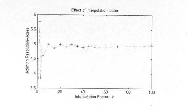
S2.C5.D1

CHAPTER 6: COMPARISION, CONCLUSION & FUTURE PATH

S2.C6.1 COMPARISION

For both Azimuth correlation approaches,

1 TASP (Time-Domain Azimuth Signal Processing) and

2 FASP (Frequency-Domain Azimuth Signal Processing)

As described in Chapter 4 and Chapter 5 with the simulated results of S2.C4.3 and S2.C5.3, and individual interpretations of S2.C4.4 and S2.C5.4, keeping in front, the relative comparison, conclusion and future path are summarized as below.

Ø TASP is suitable for sample by sample processing approach whereas FASP advocates block-processing methodology.

Ø TASP is characterized by large and redundant computations with time trade-off because of significant processing time variations for wide-swath near-to-far range conditions. FASP is characterized by less computational involvement with memory trade-off because of entire aperture data storage requirement for block-processing.

Ø TASP is ideal, model, and simpler algorithm with minimal processing artifacts. It is carried out in a single-uniform and natural domain i.e. Time. FASP is the derived form of TASP because of the inverse and bi-directional relationship between Time and Frequency. FASP is switched between time to frequency and frequency to time by mathematically bounded, finite length, discrete and less precise transformation tools like FFT and IFFT, which contribute more artifacts to the End Results.

Ø TASP gives better End Results than both the variants of FASP. It is an ideal choice to confirm and visualize the effect of processing parameter variations just using a prototype project configuration with a small data set of known pattern. FASP is generally feasible with practically acceptable tolerances for the actual implementation over a massive data set received with unknown stoic behavior.

Ø On the basis of available memory and time, the selection should be…

· Memory: Sufficiently large à FASP

Relatively less à TASP

· Time: On-line/Sample wise/Fast à TASP with Hamming weighting

Pre-stored/ Block wise /Moderate à FASP with Kaiser weighting

On-line/Block wise/Fast à FASP with Hamming weighting

Ø Data skewing effect due to Range-Walk Curvature or Range Cell Migration has to be minimized for high-resolution SAR imaging through RCMC. Since RCMC is convenient and faster to perform in Frequency-Domain for high-resolution requirement, where, there is no way to get rid of RCMC, FASP is the obvious choice.

S2.C6.2 CONCLUSION

The decision to adopt either TASP or FASP for actual Real-time implementation is mainly governed by the available hardware technology (DSP processor, Memory) with its throughput delivery speed and cost, and by the justifiable requirement/need to approach as near as possible towards Real-time processing. Expected quality and resolution of the image are also considerable driving forces.

S2.C6.3 FUTURE PATH

è Some more window functions should be explored with better Main lobe–Side lobe characteristics.

è Both TASP and FASP can be reconsidered with multiplicative speckle models.

è Simulations of other relevant issues like Motion Compensation, RCMC, Geometric and Radiometric Corrections are also equally challenging.

è Third possible Azimuth Correlation algorithm i.e., SPECAN (De-ramping) should be simulated to confirm its proposed trade-off ability with TASP and FASP.